Executive Summary
Revenue forecasting is an essential part of any retail business, and the difference between success and failure often means having a good idea of where sales will be a year down the road: Staffing, inventory, promotional planning, and the coordination of distribution channels all depend on accurate forecasting.The most common means of knowing where your business will be in the future is charting where it has been in the past. But how can you use data from a year like 2020, where lockdowns and store closures left huge holes in sales data?
An Example of Gaps in Data
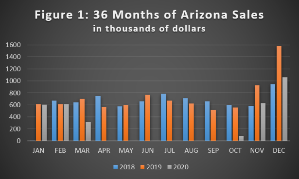
The data in Figure 1 (below) offer an example, coming from a national apparel retailer’s single store in Arizona. This store closed in mid-March of 2020 because of COVID-19, not re-opening until late October. As such, sales over these months are absent.
Below we suggest some simple yet effective ways retailers can suture their datasets so that they may make useful inferences and projections. Statisticians call the process of filling in missing data points imputation.
Method 1: Imputation Using Data from Prior Years
The most generalizable (and probably most common) type of imputing missing data is “mean substitution” and its variants, where the averages of non-missing values are used. While this is often useful and makes intuitive sense, it is not always the most useful tack as it doesn’t necessarily take into consideration the shape of your data. Revenue data is especially sensitive to seasonality, so it is important to use methods that account for this. Imagine you’re reading sheet music and a chord has gotten obscured (because, if you’re like me, you’ve spilled salsa on it). You wouldn’t necessarily substitute the “average” chord for the missing one, but instead you’d consider the structure of the song – its shape – and impute something accordingly.
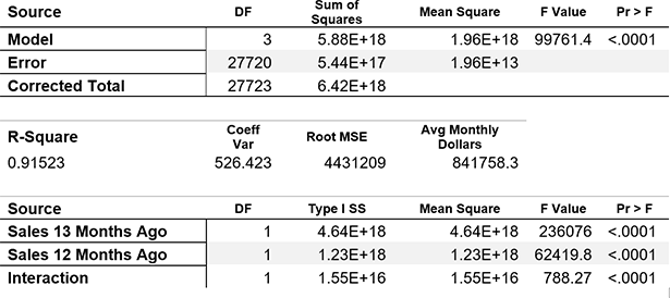
One place we might look for a substitute chord is in a similar song, and in retail data it is often the case that the most “similar song” is same-store sales from the previous year. If we look at Figure 1 above, we notice that the shape of 2019 data tracks somewhat closely (if imperfectly) with 2018 values, and in fact this holds not just for this store, but for the entire chain. Using linear regression analysis, we find that 91.5% of the variance for any given month can be accounted for by three variables: sales from 12 months earlier, sales from 13 months earlier, and the interaction between the two:
Table 1: Results of Regression Analysis
Using Sales Lagging 12th and 13th Prior Months
to Predict Monthly Dollars
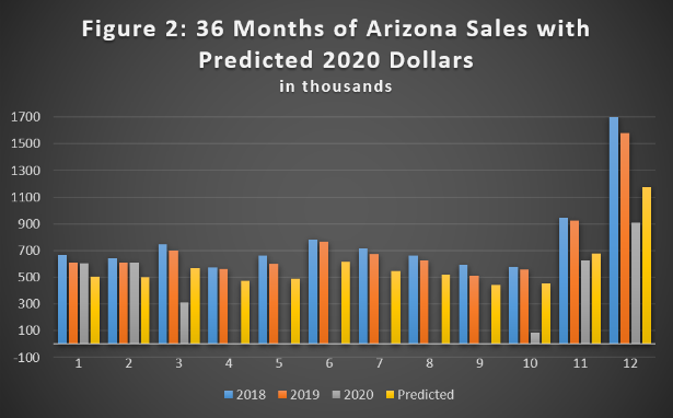
The result (in Figure 2 below) shows well-fitting predicted values for 2020 (indicated by the yellow bars). Given that data for both March and October are only partial months, the predicted values for these months can be used for projections and forecasting.
Method 2: Imputation Using Surrogate Store Data
In the Arizona store above, we had 36 months of data to work with, enabling us to verify that 2018 sales looked a lot like 2019 sales, giving us confidence that our 2020 imputations are meaningful. But what if a particular store doesn’t have historical data? Or what if a store’s historical data doesn’t yield a good prediction about its future sales? A good option is to find another store whose data we can use as a surrogate.
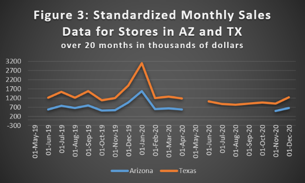
Again we use the same Arizona store, this time looking only at sales from May 2019. Looking at our data we notice that we have three incomplete months in 2020: March (15 days of sales) October (5 days), and December (25 days). Since we only have 14 months to model with, and since we’d like to use these three months’ data, we “standardize” our months by creating 30-day totals based on daily averages: We first calculate the average daily sales for each month for all of our retailer’s stores and then multiply these values by 30, giving us standard 30-day “months.”
With these standardized months we can now look for a surrogate store whose data fit our Arizona store. While typical retails chains have many stores with closures in 2020, closures were irregular and atypical: Different stores were shuttered and reopened at different times in different regions, and some stores may even have data in all twelve months of the year. The Arizona store in our example comes from a national U.S. retailer with over 1000 outlets, eight of which had sales data in 11 of 12 months in 2020. If any of these eight have monthly sales data are highly correlated with our Arizona store (i.e., they share a similar shape) then we may use it in our imputation.
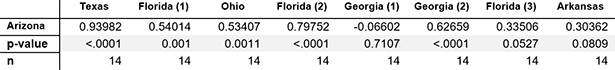
Of these eight, an excellent fit with Arizona sales is a store in Texas, which has a correlation of .95 – higher, in fact, than using same-store year-over-year sales by month. As a further measure of these two stores’ similarity, we look at an additional correlation: the percentage of all sales coming from specialty apparel (again, using standardized 30-day “months”).
As with raw monthly sales, we again see Arizona’s strongest correlation is with this same Texas store. And again, this relationship is significantly stronger than using 12-month same-store lag data, which has a correlation of .75. We have found our fit1.
Table 2: Correlation of Arizona Sales with 8 Stores
Percentage of Specialty Sales over 14 Months
1The effect of an interaction between two variables can be gotten by including their product as an additional independent variable.
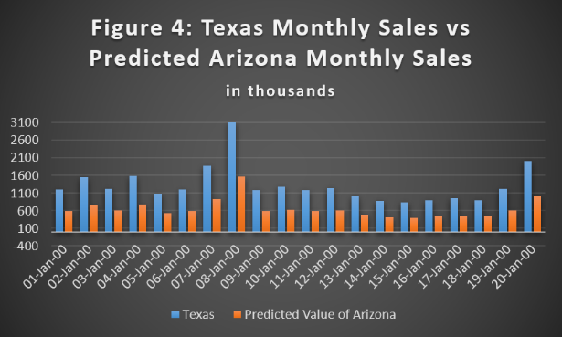
Plotting our Texas store months against our Arizona values yields this:
For months in which we have data in both stores we see a nice fit, and thus we feel good about using Texas as surrogate data for Arizona. However, we note a hole in the Texas data for May 2020. From our previous method we found we can model using lagged values from 12 and 13 months prior, which – for Texas – we have. We can thus impute this missing Texas value in our predictor data so that we can then model Arizona’s missing values. Using linear regression with one variable, we get the following nice result:
Table 3: Simple Linear Regression
Using Texas Monthly Data to Model Arizona
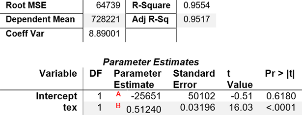
The R-Square value tells us that Texas data explains over 95% of the variance in the Arizona data, and the parameter estimates of the intercept (at “A”) and predictor (at “B”) give us an equation for filling in our missing Arizona months:
ArizonaMonth = -25621 + TexasMonth x 0.51240
Calculating the values to use in our imputation thus yields this:
Summary
There you have it: two simple methods for dealing with a complicated year. By imputing values for missing 2020 data points in a reasonable way, you should be able to make reasonable forecasts about 2021 and beyond.The Impact of COVID-19 on Key Retail Segments


Author
Chris Hanks, PhD. Director, Data Sciences, Appriss Retail
Chris Hanks is the director, data sciences, at Appriss Retail and is based in the Irvine office. Chris earned his Ph.D. in political psychology from University California, Irvine, where he was a senior predictive modeler at the UCI Center for Statistical Consulting. He spent seven years as a neuroscientist before moving to retail analytics in 2011. Chris is involved with American Statistical Association where he has held a chair position.